How the kmos kMC algorithm works
kmos asks you to describe your model to the processor in seemingly arcane ways. It can save model descriptions in XML but they are basically unreadable and a pain to edit. The API has some glitches and is probably incomplete: so why learn it?
Because it is fast (in two ways).
The code it produces is commonly faster than naive implementations of the kMC method. Most straightforwards implementations of kMC take a time proportional to 2*N per kMC step, where N is the number of sites in the system. However the code that kmos produces is O(1) until the RAM of your system is exceeded. As benchmarks have shown this may happen when 100,000 or more sites are required. However tests have also shown that kmos can be faster than O(N) implementations from around 60-100 sites. If you have different experiences please let me know but I think this gives some rule of thumb.
Why is it faster? Straightforward implementations of kMC scan the entire system twice per kMC step. First to determine the total rate, then to determine the next process to be executed. The present implementation does not. kmos keeps a database of available processes which allow to quickly pick the next process. It also updates the database of available processes which cost additional overhead. However this overhead is independent of the system’s size and only scales with the degree of interaction between sites, which is seems hard to define in general terms.
The second way reason why it is fast is because you can formulate processes in a intuitive fashion and let kmos figure how to make fast running code out of it. So we save in human time and CPU time, which is essentially human time as well. Yay!
To illustrate just how fast the algorithm is the graph below shows the CPU time needed to simulate 1 million kMC steps on a simple cubic lattice in 2 dimension with two reacting species and without lateral interaction. As this shows the CPU time spent per kMC step as nearly constant for up nearly 10^5 sites.
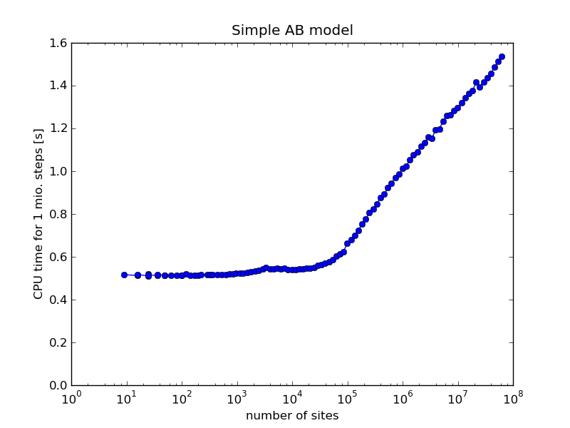
Benchmark for a simple surface reaction model. All simulations have been performed on a single CPU of Intel I7-2600K with 3.40 GHz clock speed.
The kmos O(1) solver

The data model underlying the kmos solver. The central component
is the avail_sites array which stores for each elementary
step the sites for which it is executable. Secondly
it stores the location in memory, where the availability
of the site is stored for direct access. The array of
rate constants holds the numeric rate constant and only
changes, when a physical parameter is changed. The
nr of sites array holds the total number of sites for each
process and needs to be updated whenever
a process becomes available und unavailable. The accum. rates
has to be updated once per kMC step and holds the accumulated
rate constant for each processes. That is, the last field
of accum. rates holds  ,
the total rate of the system.
,
the total rate of the system.
So what makes the kMC solver so furiously fast? The underlying data structure is shown in the picture above. The most important part is that the solver never scans the entire system for available processes except at program initialization.
Please have a look at the sketch of data structures above. Given that all arrays are initialized and populated, in each kMC step the following things happen:
In the first step we need to identify the next process and site.
To do so we draw a random number ![R_{1} \in [0, 1]](../_images/math/87b170ed9889089d6aed60224e6c43cd28b44178.png) .
This number has to be scaled to ,
so we multiply it with the last field in accum. rates. Next
we simply perform a
binary search
for the right process on accum. rates. Having determined the
process, we pick a site using a second random number
.
This number has to be scaled to ,
so we multiply it with the last field in accum. rates. Next
we simply perform a
binary search
for the right process on accum. rates. Having determined the
process, we pick a site using a second random number  ,
which is constant in time since avail sites is filled up with
the available site for each process from the left.
,
which is constant in time since avail sites is filled up with
the available site for each process from the left.
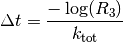
Totally independent of this we calculate the duration of the
current step with another random number  using
using
So, while the determination of process and site is extremely straightforward, the CPU intensive part just starts now. The proclist module is written in such a way, for each elementary step it updates the avail sites array only in the local neighborhood of the site, where the process is executed. It is furthermore heuristically optimized in order to require only a minimal number of if-statement to figure out which database updates are necessary. This will be explained in greate detail in the next subsection.
For the current description it is sufficient to know that for all database updates by the proclist module :
- the nr of sites array is updated as well.
- adding or deleting an available site only takes constant time, since the number of available sites as well as the memory addresses is always updated. Thus new sites are simply add at the end of the list of available sites. When a site has to be deleted the last site in the array is moved to the memory slot available now.
Thus once all local updates are finished the accum. rates array is simply updated once. And ready we are for the next kMC step.
Todo
describe translation algorithm